II – Examples
In this article, we will go through a few examples, using the different tools to explore particular splicing events.
Table of contents
II - Examples
  II-1. A simple alternative first exon: ric-4
  II-2. A more complex case: glb-17
  II-3. A complex locus: unc-43
  II-4. Novel exons: srx-45
    Potential novel cassette exon
    Potential novel first exon
  Summary
1. A simple alternative first exon: ric-4
The gene ric-4 plays an important role for synaptic vesicles. We first look at the CeNGEN scRNA-Seq data to confirm that, as can be expected for this central synaptic gene, it is highly expressed in every neuron type (and not expressed in non-neuronal tissues).

We then examine the annotated gene model in the genome browser. There are 2 annotated transcripts, with an alternative first exon (the gene is on the – strand as indicated by its color, thus the first exon is the one on the right, the last exon on the left). We also display the “maximum coverage” track, which shows evidence of expression for both of the alternative first exons.

We further examine the “maximum” splice junction track. Because this gene is highly expressed, there are many “noisy” splice junctions in the gene body. We use the Basic Display to visualize the splice junctions of interest:

[advanced usage] We could filter out the junctions to only display those with more than 100 reads by playing with the advanced track settings. This is only done here for illustration.

So, we can tell that both alternative first exons are expressed in some neurons. We don’t know at this point if every neuron expresses both transcripts, or if some neurons express one transcript preferentially. Let’s open the first neuron in the list, ADL.

ADL expresses exclusively one transcript, with the distal first exon. Indeed, in the ADL samples we detect 1,372 reads supporting the distal exon, and only 97 reads supporting the proximal exon. The exonic coverage also suggests no expression of the proximal exon.
Which neuron(s) express this proximal exon? As it is present in the “maximum” tracks, there is at least one neuron expressing it, but we don’t want to examine each neuron one by one! We switch to the Local Quantification.

In the Splice Graph, we see three “interesting” features: an intron retention between exon 1 and 2, a junction in the middle of exon 2, and an alternative first exon with exon 3 as target. We can confirm the position of our event of interest by switching to genomic scale,

or by hovering on exon 3 to see its genomic coordinates

Let’s examine the LSVs. The first one is the intron retention between exons 1 and 2. This intron retention appears green in the Splice Graph, indicating it’s not present in the annotation. In other words, when MAJIQ first examined our dataset, it saw some evidence suggesting the possibility of intron retention in this location, and added it as an alternative event.

On this schematic, the known junction is in red and the retained intron in blue. We can look at the quantification in each neuron (scroll to the right to see more neurons).

It turns out, none of these neurons display noticeable intron retention. This LSV can be safely ignored.
Now let’s switch to the more interesting LSV, the alternative first exon.

We have two junctions in this LSV, the red (corresponding to exon 1) and the blue (corresponding to exon 2). We can visualize the quantification in all neuron types, here I restricted the display to ADL, IL2, PVD, and PVM.

ADL and IL2 have strong evidence of using the red, distal exon (exon 1), PVD and PVM have strong evidence of using the blue, proximal exon (exon 2). We can confirm this by looking back at the genome browser.

Indeed, while ADL and IL2 appear to exclusively express the distal exon 1, in PVD and PVM 2/3rd of the reads correspond to the proximal exon 2.
Finally, let’s look at the transcript-level quantification. We can see from the Wormbase browser that the proximal exon 2 is included in transcript Y22F5A.3b.1, here called ric-4b, and the distal exon 1 is included in ric-4a.

Indeed, by mean transcript usage, ric-4a constitutes 90 % of expression in IL2 and ADL, and only 20-30 % in PVM and PVD.

Thus, we examined the alternative first exon of ric-4 with three tools, and find generally the same result.
2. A more complex case: glb-17
For our second example, we will consider the globin-related gene glb-17. Again, we first verify its general expression pattern in scRNA-Seq and notice a very strong expression in PVP, with lower expression in some other neurons (AUA, PVN, AVG, DVC, PQR, BDU, PLM, PHC, PVW, FLP, ALM, RIC, PVQ, URX, PVM, ALA).


Note however that not all neurons were sequenced. For example, we do not have data for AUA and PVN, but we have data for AVG and DVC.
We display the gene model, along with the “maximum” tracks and the PVP tracks (since we know this neuron will be responsible for most of the expression). The gene model contains two isoforms, differing by a 5′ splice site (at the end of the 4th exon, counting from the right), as well as two sets of transcripts with differing 5′ UTRs. Examining the tracks, the “maximum” tracks are dominated by PVP (as expected). The PVP splice junction track is extremely noisy and hard to interpret, due to the very high expression of this gene in this cell type.

The local quantification describes 3 LSVs. The first LSV has exon 1 (inside the 5’UTR) as a source. It considers in blue the annotated junction to exon 2, in red a novel, shorter junction (i.e. alternative 3′ splice site) making exon 2 longer, in green, the skipping of exon 2, jumping to exon 3, and in purple an intron retention making exon 1 and 2 part of a single long exon.

This LSV was only quantified in PVP and DVC, which both display 75-80 % usage of the blue, annotated, junction.

However, recall that, from scRNA-Seq, we expect measurable expression of glb-17 in AVG, but our local quantification tool does not measure this LSV in AVG. We can go back to the genome browser and open the AVG tracks to better understand.

While there may be (gene) expression of glb-17 in AVG, this first exon isn’t expressed. This does not appear in an LSV: LSVs capture the preferential usage of one junction compared to others. Here there is no junction usage to work with, we do not have any quantification. To examine this, we need to use the transcript-level quantification.

In terms of relative usage, AVG only expresses F49E2.4a.2 and F49E2.4b.2 (which do not include exon 1), and not the .1 variants (which do include exon 1).
Continuing with the local quantifications, our second LSV with exon 3 as target does not display differential usage in practice (and is not annotated in Wormbase), we can discount it as a false positive.

Finally, the third LSV accounts for the alternative 5′ splice site at the end of exon 4. Based on the quantifications, our 3 neurons of interest use a balance of both junctions.


This can be confirmed in the genome browser: we have a similar usage of both splice sites (note, for legibility, I hid part of the PVP_sj track in this image).

This observation is consistent with the transcript-level quantification: in all three neurons, we observe similar proportions of F49E2.4a.n and F49E2.4b.n (where n is either 1 or 2).
3. A complex locus: unc-43
There are at least 140 genes with 10 or more annotated transcripts (e.g. etr-1, mvk-1, fln-2, …). Interpreting their splicing patterns is hard. We will take a look at unc-43/CaMKII to illustrate some ways to approach its analysis. First, let’s visualize the full locus.

We can distinguish several groups of transcripts. Most transcripts share a group of 3′ exons, with various first exons. Many transcripts share the central group of exon in addition. A smaller group of transcripts, at the bottom, use this central group as their 3′ end.
We notice that some transcripts are distinguished by long UTRs (annotated in maroon) but overlap with a CDS. From RNA-Seq data, we can not distinguish those: we can only determine if this sequence is expressed, not if it’s coding. However for these transcripts to express the same region but not translate it, there has to be a frame-shift somewhere upstream, typically an alternative splice site, which we can measure (on the left image, we see two transcripts with a long 3′ UTR; on the right we zoomed in on one exon and see how an alternative 3′ splice site induced a frame-shift and an early stop codon, thus starting the 3′ UTR).


This alternative splice site can be directly interrogated in the local quantification. By zooming in in the genome browser we can determine its coordinates: we are interested in the splice junction 10,334,127-10,329,195 which is part of the target LSV into exon 19, the grey junction from exon 14.


We can then examine the relative usage of this junction within the LSV, it appears RMD has a relatively higher usage of this alternative splice site.
We can use a similar approach to compare the alternative first exons: we need to locate the LSV that distinguishes two alternative first exons and compare the junction usage.
A more challenging case arises when we try to interrogate the 5′-most exon. Its inclusion is not reflected in any LSV, as it does not arise from a “choice” between two splice junctions: exon 2 either is the first exon of the transcript, or it’s the second. Thus in this case the local quantification cannot help us.

In principle, the transcript-level quantification can provide an answer, as it does take exonic reads into account. However, in a complex gene such as unc-43, three problems arise: first, the plots quickly become unreadable because of the amount of data, second we run out of colors and some transcripts are not plotted at all, third because the reads may get “diluted” across all these transcripts the quantifications may become more noisy. In the case of unc-43, an examination of the gene model shows us that this first exon is specific to transcript K11E8.1r.1, but this transcript is not visibly plotted because we ran out of colors.

To circumvent this problem, we can open the heatmap, plot unc-43 and download the table.

We can then open this table in Excel and filter and sort to find the neurons with highest expression of the transcript unc-43r, in this case RIA, PVD and PVM.

We then verify this expression in the genome browser (here along with LUA as an example of neuron with low expression of unc-43r). We notice that this exon is only supported by 15 reads, as opposed to more than 1000 reads for junctions inside the gene body: we should be highly skeptical.

4. Novel exons: srx-45
Next we will take the example of the GPCR srx-45. As usual we start by examining its expression in scRNA-Seq. It is expressed only in a restricted set of neurons, most highly in AIM, PHB, M5, PVT, I2, ASH, I4, M2, AVJ, AIN, and M4. Of these neurons, we have sequencing data for AIM, AIN and M4. Note however that M4 was sequenced with a single biological replicate, making it less reliable.

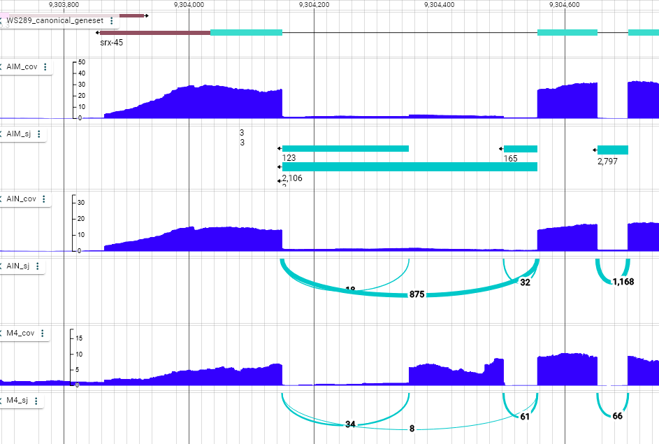
Examining the annotated gene model shows a single transcript. However, looking at the “maximum” tracks shows 2 notable potential inconsistencies (we will ignore the 42 reads skipping the second exon end, and the 32 reads forming an alternative splice site in the middle, as these are low number of reads compared to the rest of the gene).

The first notable element looks like an alternative cassette exon in penultimate position, the other is the splice junction upstream of the first exon, suggesting the existence of an alternative (or constitutive) first exon.

Potential novel cassette exon
These two splice junctions appear to delinate a novel, unannotated, cassette exon.

Would inclusion of this exon affect the protein sequence of SRX-45? We zoom in on this region and display the “Reference sequence” track. The track itself is composed of 8 sequences stacked. The 4th one (TTTTTACTAA…GGGGTGTT) is the reference genomic DNA sequence. Above are the 3 translations of this sequence in the three possible frames. Below this genomic sequence is its reverse complement, i.e. the genomic sequence of the – strand, along with its 3 translations. Note that, in the translations, potential start codons are highlighted in green, potential stop codons in red.

Since the gene srx-45 is on the – strand, we need to read the bottom half of this track. We will zoom out a bit to have the entire potential novel exon visible.

By examining the three bottom translations, we notice that all of them contain a stop codon within this exon! It cannot be inserted in the protein without disrupting it.
Is the sequencing data wrong? We can open the “neurons” track from the Koterniak (2020) TRAP-Seq data, which supports the existence of these splice junctions.

Finally, we can open the Wormbase browser at the same coordinates and display the following tracks:
- RNASeq
- RNASeq Splice Junctions (common)
- UCSC Conservation
- Nanopore matches

These tracks all support the existence of an exonic region at this location. We will not question this exon further here, and focus on its expression pattern assuming it is a “normal” cassette exon.
In the local quantification module, we first look at the Splice Graph. Here we are interested in exon 8, which appears in green as it is not an annotated exon.

Since it’s a cassette exon, we need to look at two LSVs, the source LSV from exon 7 and the target LSV into exon 9.
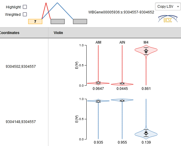

This suggests that this cassette exon is included specifically in M4, and skipped in AIM and AIN. This is consistent with what we observe in the genome browser.
And what about the transcript-level quantification?

The transcript-level quantification is only based on annotated transcripts (in WS289). Thus it’s not aware of any potential novel exon and won’t display them.
Potential novel first exon
Second, we can examine the potential novel first exon.

We notice that the corresponding junction is unusually long: clicking on the junction opens a panel on the right, indicating this junction is almost 5 kb long! While such long introns do exist in the genome, they are not common (1,681 out of 204,438 in WS289, this intron would be in the top 0.8 % longest).

As with the cassette exon, one immediate question is whether it is compatible with the srx-45 ORF. We first need to determine the frame. We zoom in on the beginning of the annotated gene and display the “Reference sequence” track. Note that since this gene is on the – strand, we need to look at the bottom half of the Reference sequence track.

We notice that the Wormbase annotation starts on ATG without 5′ UTR, with the (green) Methionine starting the ORF. Thus, the correct frame is the top one, and the protein sequence (from left to right) is MFQILMENV… To confirm this, we can click on the gene model in the “canonical geneset” track, this opens a panel, in which we can click on the gene name to open the Wormbase page and double-check the protein sequence.

Considering the position of the splice junction, the first base pairs after the intron are ATTCTC, which are in frame. We can now move to the novel first exon and examine the sequence upstream of the intron.

The bottom frame is the correct one (if we had an overhang, we would be frame-shifted when we arrive in the annotated exon), and indeed we have a Methionine and no stop codon. Thus, assuming this novel first exon is real, it leads to an alternative protein N terminus:
SRX-45 annotated:  MFQILMENV...
SRX-45 novel    :    MILMENV...
One additional note: examining the amount of RNA-Seq in the annotated first exon, we notice a very low coverage of the first few base pairs. This may lead us to speculate that there might be a short 5′ UTR and the correct start codon is the second Methionine (thus the sequence of the protein would start with MENV…).
As with the cassette exon, we can examine the evidence available in Wormbase. We open the browser with the “Trans-spliced acceptor” track in addition to the previous ones.

The evidence supports the existence of this novel first exon. In addition, we can load our track in the UCSC browser along with Durham et al.‘s scATAC-Seq data (detailed in part III), and we notice regions of open chromatin in neurons around the location of this exon (srx-45 is annotated K01B6.2 in this screenshot).

Overall this evidence supports the existence of this novel exon. Which leads us to the next question: in which neuron(s) is it expressed? Again, the transcript-level quantification is only aware of annotated transcripts, and won’t help us here. Further, when we look at the Splice Graph in the local quantification, we do not see this exon (here we switched the Splice Graph representation to genomic coordinates, making it obvious that we don’t have a 5 kb splice junction).

So we can’t rely on the local quantification in this case. We know (from the scRNA-Seq) that this gene is expressed highly only in a few neurons (notably AIM, AIN and M4), thus it is convenient enough to just open the tracks for these neurons, in which it appears this exon is expressed AIN, partially in AIM, and not in M4.

Summary
- Before analyzing alternative splicing, we look at the gene expression in scRNA-Seq data
- Every analysis starts with the genome browser, using the “maximum” tracks to get a general idea of the transcript structure
- The local quantification then allows us to look at individual LSVs across all neurons
- The local quantification typically contains many “false positives”, potential events that do not actually vary between neurons
- The transcript-level quantification is sometimes more readable (not always)
- The local quantification can be used to compare alternative splice junction usage. If we have an optional exon without alternative, we can sometimes detect it in the transcript-level quantification, or in the genome browser
- The last step of every analysis is to confirm our observations in the genome browser
- There are many potential novel exons. We can typically look at their effect on the ORF and use external data (conservation, Nanopore, …) to assess their existence